System of linear equations

A linear system in three variables determines a collection ofplanes.The intersection point is the solution.

Inmathematics,asystem of linear equations(orlinear system) is a collection of two or morelinear equationsinvolving the samevariables. For example,

${\begin{cases}3x+2y-z=1\\2x-2y+4z=-2\\-x+{\frac {1}{2}}y-z=0\end{cases}}$

is a system of three equations in the three variablesx,y,z.Asolutionto a linear system is an assignment of values to the variables such that all the equations are simultaneously satisfied. In the example above, a solution is given by theordered triple $(x,y,z)=(1,-2,-2),$ since it makes all three equations valid.

Linear systems are a fundamental part oflinear algebra,a subject used in most modern mathematics. Computationalalgorithmsfor finding the solutions are an important part ofnumerical linear algebra,and play a prominent role inengineering,physics,chemistry,computer science,andeconomics.Asystem of non-linear equationscan often beapproximatedby a linear system (seelinearization), a helpful technique when making amathematical modelorcomputer simulationof a relativelycomplex system.

Very often, and in this article, thecoefficientsand solutions of the equations are constrained to berealorcomplex numbers,but the theory and algorithms apply to coefficients and solutions in anyfield.For otheralgebraic structures,other theories have been developed. For coefficients and solutions in anintegral domain,such as theringofintegers,seeLinear equation over a ring.For coefficients and solutions that are polynomials, seeGröbner basis.For finding the "best" integer solutions among many, seeInteger linear programming.For an example of a more exotic structure to which linear algebra can be applied, seeTropical geometry.

Elementary examples

Trivial example

The system of one equation in one unknown

$2x=4$

has the solution

$x=2.$

However, most interesting linear systems have at least two equations.

Simple nontrivial example

The simplest kind of nontrivial linear system involves two equations and two variables:

${\begin{alignedat}{5}2x&&\;+\;&&3y&&\;=\;&&6&\\4x&&\;+\;&&9y&&\;=\;&&15&.\end{alignedat}}$

One method for solving such a system is as follows. First, solve the top equation for$x$in terms of$y$:

$x=3-{\frac {3}{2}}y.$

Nowsubstitutethis expression forxinto the bottom equation:

$4\left(3-{\frac {3}{2}}y\right)+9y=15.$

This results in a single equation involving only the variable$y$.Solving gives$y=1$,and substituting this back into the equation for$x$yields$x={\frac {3}{2}}$.This method generalizes to systems with additional variables (see "elimination of variables" below, or the article onelementary algebra.)

General form

A general system ofmlinear equations withnunknownsandcoefficientscan be written as

${\begin{cases}a_{11}x_{1}+a_{12}x_{2}+\dots +a_{1n}x_{n}=b_{1}\\a_{21}x_{1}+a_{22}x_{2}+\dots +a_{2n}x_{n}=b_{2}\\\vdots \\a_{m1}x_{1}+a_{m2}x_{2}+\dots +a_{mn}x_{n}=b_{m},\end{cases}}$

where$x_{1},x_{2},\dots,x_{n}$are the unknowns,$a_{11},a_{12},\dots,a_{mn}$are the coefficients of the system, and$b_{1},b_{2},\dots,b_{m}$are the constant terms.

Often the coefficients and unknowns arerealorcomplex numbers,butintegersandrational numbersare also seen, as are polynomials and elements of an abstractalgebraic structure.

Vector equation

One extremely helpful view is that each unknown is a weight for acolumn vectorin alinear combination.

$x_{1}{\begin{bmatrix}a_{11}\\a_{21}\\\vdots \\a_{m1}\end{bmatrix}}+x_{2}{\begin{bmatrix}a_{12}\\a_{22}\\\vdots \\a_{m2}\end{bmatrix}}+\dots +x_{n}{\begin{bmatrix}a_{1n}\\a_{2n}\\\vdots \\a_{mn}\end{bmatrix}}={\begin{bmatrix}b_{1}\\b_{2}\\\vdots \\b_{m}\end{bmatrix}}$

This allows all the language and theory ofvector spaces(or more generally,modules) to be brought to bear. For example, the collection of all possible linear combinations of the vectors on the left-hand side is called theirspan,and the equations have a solution just when the right-hand vector is within that span. If every vector within that span has exactly one expression as a linear combination of the given left-hand vectors, then any solution is unique. In any event, the span has abasisoflinearly independentvectors that do guarantee exactly one expression; and the number of vectors in that basis (itsdimension) cannot be larger thanmorn,but it can be smaller. This is important because if we havemindependent vectors a solution is guaranteed regardless of the right-hand side, and otherwise not guaranteed.

Matrix equation

The vector equation is equivalent to amatrixequation of the form $$A\mathbf {x} =\mathbf {b}$$ whereAis anm×nmatrix,xis acolumn vectorwithnentries, andbis a column vector withmentries.

$$A={\begin{bmatrix}a_{11}&a_{12}&\cdots &a_{1n}\\a_{21}&a_{22}&\cdots &a_{2n}\\\vdots &\vdots &\ddots &\vdots \\a_{m1}&a_{m2}&\cdots &a_{mn}\end{bmatrix}},\quad \mathbf {x} ={\begin{bmatrix}x_{1}\\x_{2}\\\vdots \\x_{n}\end{bmatrix}},\quad \mathbf {b} ={\begin{bmatrix}b_{1}\\b_{2}\\\vdots \\b_{m}\end{bmatrix}}.$$ The number of vectors in a basis for the span is now expressed as therankof the matrix.

Solution set

The solution set for the equationsx−y= −1and3x+y= 9is the single point (2, 3).

Asolutionof a linear system is an assignment of values to the variablesx₁,x₂,...,x_nsuch that each of the equations is satisfied. Thesetof all possible solutions is called thesolution set.

A linear system may behave in any one of three possible ways:

1. The system hasinfinitely many solutions.
2. The system has aunique solution.
3. The system hasno solution.

Geometric interpretation

For a system involving two variables (xandy), each linear equation determines alineon thexy-plane.Because a solution to a linear system must satisfy all of the equations, the solution set is theintersectionof these lines, and is hence either a line, a single point, or theempty set.

For three variables, each linear equation determines aplaneinthree-dimensional space,and the solution set is the intersection of these planes. Thus the solution set may be a plane, a line, a single point, or the empty set. For example, as three parallel planes do not have a common point, the solution set of their equations is empty; the solution set of the equations of three planes intersecting at a point is single point; if three planes pass through two points, their equations have at least two common solutions; in fact the solution set is infinite and consists in all the line passing through these points.

Fornvariables, each linear equation determines ahyperplaneinn-dimensional space.The solution set is the intersection of these hyperplanes, and is aflat,which may have any dimension lower thann.

General behavior

The solution set for two equations in three variables is, in general, a line.

In general, the behavior of a linear system is determined by the relationship between the number of equations and the number of unknowns. Here, "in general" means that a different behavior may occur for specific values of the coefficients of the equations.

• In general, a system with fewer equations than unknowns has infinitely many solutions, but it may have no solution. Such a system is known as anunderdetermined system.
• In general, a system with the same number of equations and unknowns has a single unique solution.
• In general, a system with more equations than unknowns has no solution. Such a system is also known as anoverdetermined system.

In the first case, thedimensionof the solution set is, in general, equal ton−m,wherenis the number of variables andmis the number of equations.

The following pictures illustrate this trichotomy in the case of two variables:

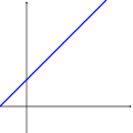
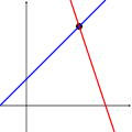
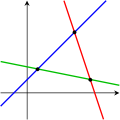
One equation	Two equations	Three equations

The first system has infinitely many solutions, namely all of the points on the blue line. The second system has a single unique solution, namely the intersection of the two lines. The third system has no solutions, since the three lines share no common point.

It must be kept in mind that the pictures above show only the most common case (the general case). It is possible for a system of two equations and two unknowns to have no solution (if the two lines are parallel), or for a system of three equations and two unknowns to be solvable (if the three lines intersect at a single point).

A system of linear equations behave differently from the general case if the equations arelinearly dependent,or if it isinconsistentand has no more equations than unknowns.

Properties

Independence

The equations of a linear system areindependentif none of the equations can be derived algebraically from the others. When the equations are independent, each equation contains new information about the variables, and removing any of the equations increases the size of the solution set. For linear equations, logical independence is the same aslinear independence.

The equationsx− 2y= −1,3x+ 5y= 8,and4x+ 3y= 7are linearly dependent.

For example, the equations

$3x+2y=6\;\;\;\;{\text{and}}\;\;\;\;6x+4y=12$

are not independent — they are the same equation when scaled by a factor of two, and they would produce identical graphs. This is an example of equivalence in a system of linear equations.

For a more complicated example, the equations

${\begin{alignedat}{5}x&&\;-\;&&2y&&\;=\;&&-1&\\3x&&\;+\;&&5y&&\;=\;&&8&\\4x&&\;+\;&&3y&&\;=\;&&7&\end{alignedat}}$

are not independent, because the third equation is the sum of the other two. Indeed, any one of these equations can be derived from the other two, and any one of the equations can be removed without affecting the solution set. The graphs of these equations are three lines that intersect at a single point.

Consistency

See also:Consistent and inconsistent equations

The equations3x+ 2y= 6and3x+ 2y= 12are inconsistent.

A linear system isinconsistentif it has no solution, and otherwise, it is said to beconsistent.When the system is inconsistent, it is possible to derive acontradictionfrom the equations, that may always be rewritten as the statement0 = 1.

For example, the equations

$3x+2y=6\;\;\;\;{\text{and}}\;\;\;\;3x+2y=12$

are inconsistent. In fact, by subtracting the first equation from the second one and multiplying both sides of the result by 1/6, we get0 = 1.The graphs of these equations on thexy-plane are a pair ofparallellines.

It is possible for three linear equations to be inconsistent, even though any two of them are consistent together. For example, the equations

${\begin{alignedat}{7}x&&\;+\;&&y&&\;=\;&&1&\\2x&&\;+\;&&y&&\;=\;&&1&\\3x&&\;+\;&&2y&&\;=\;&&3&\end{alignedat}}$

are inconsistent. Adding the first two equations together gives3x+ 2y= 2,which can be subtracted from the third equation to yield0 = 1.Any two of these equations have a common solution. The same phenomenon can occur for any number of equations.

In general, inconsistencies occur if the left-hand sides of the equations in a system are linearly dependent, and the constant terms do not satisfy the dependence relation. A system of equations whose left-hand sides are linearly independent is always consistent.

Putting it another way, according to theRouché–Capelli theorem,any system of equations (overdetermined or otherwise) is inconsistent if therankof theaugmented matrixis greater than the rank of thecoefficient matrix.If, on the other hand, the ranks of these two matrices are equal, the system must have at least one solution. The solution is unique if and only if the rank equals the number of variables. Otherwise the general solution haskfree parameters wherekis the difference between the number of variables and the rank; hence in such a case there is an infinitude of solutions. The rank of a system of equations (that is, the rank of the augmented matrix) can never be higher than [the number of variables] + 1, which means that a system with any number of equations can always be reduced to a system that has a number ofindependent equationsthat is at most equal to [the number of variables] + 1.

Equivalence

Two linear systems using the same set of variables areequivalentif each of the equations in the second system can be derived algebraically from the equations in the first system, and vice versa. Two systems are equivalent if either both are inconsistent or each equation of each of them is a linear combination of the equations of the other one. It follows that two linear systems are equivalent if and only if they have the same solution set.

Solving a linear system

There are severalalgorithmsforsolvinga system of linear equations.

Describing the solution

When the solution set is finite, it is reduced to a single element. In this case, the unique solution is described by a sequence of equations whose left-hand sides are the names of the unknowns and right-hand sides are the corresponding values, for example$(x=3,\;y=-2,\;z=6)$.When an order on the unknowns has been fixed, for example thealphabetical orderthe solution may be described as avectorof values, like$(3,\,-2,\,6)$for the previous example.

To describe a set with an infinite number of solutions, typically some of the variables are designated asfree(orindependent,or asparameters), meaning that they are allowed to take any value, while the remaining variables aredependenton the values of the free variables.

For example, consider the following system:

${\begin{alignedat}{7}x&&\;+\;&&3y&&\;-\;&&2z&&\;=\;&&5&\\3x&&\;+\;&&5y&&\;+\;&&6z&&\;=\;&&7&\end{alignedat}}$

The solution set to this system can be described by the following equations:

$x=-7z-1\;\;\;\;{\text{and}}\;\;\;\;y=3z+2{\text{.}}$

Herezis the free variable, whilexandyare dependent onz.Any point in the solution set can be obtained by first choosing a value forz,and then computing the corresponding values forxandy.

Each free variable gives the solution space onedegree of freedom,the number of which is equal to thedimensionof the solution set. For example, the solution set for the above equation is a line, since a point in the solution set can be chosen by specifying the value of the parameterz.An infinite solution of higher order may describe a plane, or higher-dimensional set.

Different choices for the free variables may lead to different descriptions of the same solution set. For example, the solution to the above equations can alternatively be described as follows:

$y=-{\frac {3}{7}}x+{\frac {11}{7}}\;\;\;\;{\text{and}}\;\;\;\;z=-{\frac {1}{7}}x-{\frac {1}{7}}{\text{.}}$

Herexis the free variable, andyandzare dependent.

Elimination of variables

The simplest method for solving a system of linear equations is to repeatedly eliminate variables. This method can be described as follows:

1. In the first equation, solve for one of the variables in terms of the others.
2. Substitute this expression into the remaining equations. This yields a system of equations with one fewer equation and unknown.
3. Repeat steps 1 and 2 until the system is reduced to a single linear equation.
4. Solve this equation, and then back-substitute until the entire solution is found.

For example, consider the following system:

${\begin{cases}x+3y-2z=5\\3x+5y+6z=7\\2x+4y+3z=8\end{cases}}$

Solving the first equation forxgives$x=5+2z-3y$,and plugging this into the second and third equation yields

${\begin{cases}y=3z+2\\y={\tfrac {7}{2}}z+1\end{cases}}$

Since the LHS of both of these equations equaly,equating the RHS of the equations. We now have:

${\begin{aligned}3z+2={\tfrac {7}{2}}z+1\\\Rightarrow z=2\end{aligned}}$

Substitutingz= 2 into the second or third equation givesy= 8, and the values ofyandzinto the first equation yieldsx= −15. Therefore, the solution set is the ordered triple$(x,y,z)=(-15,8,2)$.

Row reduction

Main article:Gaussian elimination

Inrow reduction(also known asGaussian elimination), the linear system is represented as anaugmented matrix

$\left[{\begin{array}{rrr|r}1&3&-2&5\\3&5&6&7\\2&4&3&8\end{array}}\right]{\text{.}}$

This matrix is then modified usingelementary row operationsuntil it reachesreduced row echelon form.There are three types of elementary row operations:

Type 1:Swap the positions of two rows.

Type 2:Multiply a row by a nonzeroscalar.

Type 3:Add to one row a scalar multiple of another.

Because these operations are reversible, the augmented matrix produced always represents a linear system that is equivalent to the original.

There are several specific algorithms to row-reduce an augmented matrix, the simplest of which areGaussian eliminationandGauss–Jordan elimination.The following computation shows Gauss–Jordan elimination applied to the matrix above:

${\begin{aligned}\left[{\begin{array}{rrr|r}1&3&-2&5\\3&5&6&7\\2&4&3&8\end{array}}\right]&\sim \left[{\begin{array}{rrr|r}1&3&-2&5\\0&-4&12&-8\\2&4&3&8\end{array}}\right]\sim \left[{\begin{array}{rrr|r}1&3&-2&5\\0&-4&12&-8\\0&-2&7&-2\end{array}}\right]\sim \left[{\begin{array}{rrr|r}1&3&-2&5\\0&1&-3&2\\0&-2&7&-2\end{array}}\right]\\&\sim \left[{\begin{array}{rrr|r}1&3&-2&5\\0&1&-3&2\\0&0&1&2\end{array}}\right]\sim \left[{\begin{array}{rrr|r}1&3&-2&5\\0&1&0&8\\0&0&1&2\end{array}}\right]\sim \left[{\begin{array}{rrr|r}1&3&0&9\\0&1&0&8\\0&0&1&2\end{array}}\right]\sim \left[{\begin{array}{rrr|r}1&0&0&-15\\0&1&0&8\\0&0&1&2\end{array}}\right].\end{aligned}}$

The last matrix is in reduced row echelon form, and represents the systemx= −15,y= 8,z= 2.A comparison with the example in the previous section on the algebraic elimination of variables shows that these two methods are in fact the same; the difference lies in how the computations are written down.

Cramer's rule

Main article:Cramer's rule

Cramer's ruleis an explicit formula for the solution of a system of linear equations, with each variable given by a quotient of twodeterminants.For example, the solution to the system

${\begin{alignedat}{7}x&\;+&\;3y&\;-&\;2z&\;=&\;5\\3x&\;+&\;5y&\;+&\;6z&\;=&\;7\\2x&\;+&\;4y&\;+&\;3z&\;=&\;8\end{alignedat}}$

is given by

$x={\frac {\,{\begin{vmatrix}5&3&-2\\7&5&6\\8&4&3\end{vmatrix}}\,}{\,{\begin{vmatrix}1&3&-2\\3&5&6\\2&4&3\end{vmatrix}}\,}},\;\;\;\;y={\frac {\,{\begin{vmatrix}1&5&-2\\3&7&6\\2&8&3\end{vmatrix}}\,}{\,{\begin{vmatrix}1&3&-2\\3&5&6\\2&4&3\end{vmatrix}}\,}},\;\;\;\;z={\frac {\,{\begin{vmatrix}1&3&5\\3&5&7\\2&4&8\end{vmatrix}}\,}{\,{\begin{vmatrix}1&3&-2\\3&5&6\\2&4&3\end{vmatrix}}\,}}.$

For each variable, the denominator is the determinant of thematrix of coefficients,while the numerator is the determinant of a matrix in which one column has been replaced by the vector of constant terms.

Though Cramer's rule is important theoretically, it has little practical value for large matrices, since the computation of large determinants is somewhat cumbersome. (Indeed, large determinants are most easily computed using row reduction.) Further, Cramer's rule has very poor numerical properties, making it unsuitable for solving even small systems reliably, unless the operations are performed in rational arithmetic with unbounded precision.

Matrix solution

If the equation system is expressed in the matrix form$A\mathbf {x} =\mathbf {b}$,the entire solution set can also be expressed in matrix form. If the matrixAis square (hasmrows andn=mcolumns) and has full rank (allmrows are independent), then the system has a unique solution given by

$\mathbf {x} =A^{-1}\mathbf {b}$

where$A^{-1}$is theinverseofA.More generally, regardless of whetherm=nor not and regardless of the rank ofA,all solutions (if any exist) are given using theMoore–Penrose inverseofA,denoted$A^{+}$,as follows:

$\mathbf {x} =A^{+}\mathbf {b} +\left(I-A^{+}A\right)\mathbf {w}$

where$\mathbf {w}$is a vector of free parameters that ranges over all possiblen×1 vectors. A necessary and sufficient condition for any solution(s) to exist is that the potential solution obtained using$\mathbf {w} =\mathbf {0}$satisfy$A\mathbf {x} =\mathbf {b}$— that is, that$AA^{+}\mathbf {b} =\mathbf {b}.$If this condition does not hold, the equation system is inconsistent and has no solution. If the condition holds, the system is consistent and at least one solution exists. For example, in the above-mentioned case in whichAis square and of full rank,$A^{+}$simply equals$A^{-1}$and the general solution equation simplifies to

$\mathbf {x} =A^{-1}\mathbf {b} +\left(I-A^{-1}A\right)\mathbf {w} =A^{-1}\mathbf {b} +\left(I-I\right)\mathbf {w} =A^{-1}\mathbf {b}$

as previously stated, where$\mathbf {w}$has completely dropped out of the solution, leaving only a single solution. In other cases, though,$\mathbf {w}$remains and hence an infinitude of potential values of the free parameter vector$\mathbf {w}$give an infinitude of solutions of the equation.

Other methods

Further information:Numerical solution of linear systems

While systems of three or four equations can be readily solved by hand (seeCracovian), computers are often used for larger systems. The standard algorithm for solving a system of linear equations is based on Gaussian elimination with some modifications. Firstly, it is essential to avoid division by small numbers, which may lead to inaccurate results. This can be done by reordering the equations if necessary, a process known aspivoting.Secondly, the algorithm does not exactly do Gaussian elimination, but it computes theLU decompositionof the matrixA.This is mostly an organizational tool, but it is much quicker if one has to solve several systems with the same matrixAbut different vectorsb.

If the matrixAhas some special structure, this can be exploited to obtain faster or more accurate algorithms. For instance, systems with asymmetricpositive definitematrix can be solved twice as fast with theCholesky decomposition.Levinson recursionis a fast method forToeplitz matrices.Special methods exist also for matrices with many zero elements (so-calledsparse matrices), which appear often in applications.

A completely different approach is often taken for very large systems, which would otherwise take too much time or memory. The idea is to start with an initial approximation to the solution (which does not have to be accurate at all), and to change this approximation in several steps to bring it closer to the true solution. Once the approximation is sufficiently accurate, this is taken to be the solution to the system. This leads to the class ofiterative methods.For some sparse matrices, the introduction of randomness improves the speed of the iterative methods.One example of an iterative method is theJacobi method,where the matrix$A$is split into its diagonal component$D$and its non-diagonal component$L+U$.An initial guess${\mathbf {x}}^{(0)}$is used at the start of the algorithm. Each subsequent guess is computed using the iterative equation:

${\mathbf {x}}^{(k+1)}=D^{-1}({\mathbf {b}}-(L+U){\mathbf {x}}^{(k)})$

When the difference between guesses${\mathbf {x}}^{(k)}$and${\mathbf {x}}^{(k+1)}$is sufficiently small, the algorithm is said to haveconvergedon the solution.

There is also aquantum algorithm for linear systems of equations.

Homogeneous systems

See also:Homogeneous differential equation

A system of linear equations ishomogeneousif all of the constant terms are zero:

${\begin{alignedat}{7}a_{11}x_{1}&&\;+\;&&a_{12}x_{2}&&\;+\cdots +\;&&a_{1n}x_{n}&&\;=\;&&&0\\a_{21}x_{1}&&\;+\;&&a_{22}x_{2}&&\;+\cdots +\;&&a_{2n}x_{n}&&\;=\;&&&0\\&&&&&&&&&&\vdots \;\ &&&\\a_{m1}x_{1}&&\;+\;&&a_{m2}x_{2}&&\;+\cdots +\;&&a_{mn}x_{n}&&\;=\;&&&0.\\\end{alignedat}}$

A homogeneous system is equivalent to a matrix equation of the form

$A\mathbf {x} =\mathbf {0}$

whereAis anm×nmatrix,xis a column vector withnentries, and0is thezero vectorwithmentries.

Homogeneous solution set

Every homogeneous system has at least one solution, known as thezero(ortrivial) solution, which is obtained by assigning the value of zero to each of the variables. If the system has anon-singular matrix(det(A) ≠ 0) then it is also the only solution. If the system has a singular matrix then there is a solution set with an infinite number of solutions. This solution set has the following additional properties:

1. Ifuandvare twovectorsrepresenting solutions to a homogeneous system, then the vector sumu+vis also a solution to the system.
2. Ifuis a vector representing a solution to a homogeneous system, andris anyscalar,thenruis also a solution to the system.

These are exactly the properties required for the solution set to be alinear subspaceofRⁿ.In particular, the solution set to a homogeneous system is the same as thenull spaceof the corresponding matrixA.

Relation to nonhomogeneous systems

There is a close relationship between the solutions to a linear system and the solutions to the corresponding homogeneous system:

$A\mathbf {x} =\mathbf {b} \qquad {\text{and}}\qquad A\mathbf {x} =\mathbf {0}.$

Specifically, ifpis any specific solution to the linear systemAx=b,then the entire solution set can be described as

$\left\{\mathbf {p} +\mathbf {v}:\mathbf {v} {\text{ is any solution to }}A\mathbf {x} =\mathbf {0} \right\}.$

Geometrically, this says that the solution set forAx=bis atranslationof the solution set forAx=0.Specifically, theflatfor the first system can be obtained by translating thelinear subspacefor the homogeneous system by the vectorp.

This reasoning only applies if the systemAx=bhas at least one solution. This occurs if and only if the vectorblies in theimageof thelinear transformationA.

See also

• Arrangement of hyperplanes
• Iterative refinement
• Coates graph
• LAPACK(the free standard package to solve linear equations numerically; available inFortran,C,C++)
• Linear equation over a ring
• Linear least squares
• Matrix decomposition
• Matrix splitting
• NAG Numerical Library(NAG Library versions of LAPACK solvers)
• Rybicki Press algorithm
• Simultaneous equations

Bibliography

• Anton, Howard (1987),Elementary Linear Algebra(5th ed.), New York:Wiley,ISBN0-471-84819-0
• Beauregard, Raymond A.; Fraleigh, John B. (1973),A First Course In Linear Algebra: with Optional Introduction to Groups, Rings, and Fields,Boston:Houghton Mifflin Company,ISBN0-395-14017-X
• Burden, Richard L.; Faires, J. Douglas (1993),Numerical Analysis(5th ed.), Boston:Prindle, Weber and Schmidt,ISBN0-534-93219-3
• Cullen, Charles G. (1990),Matrices and Linear Transformations,MA: Dover,ISBN978-0-486-66328-9
• Golub, Gene H.; Van Loan, Charles F. (1996),Matrix Computations(3rd ed.), Baltimore:Johns Hopkins University Press,ISBN0-8018-5414-8
• Harper, Charlie (1976),Introduction to Mathematical Physics,New Jersey:Prentice-Hall,ISBN0-13-487538-9
• Harrow, Aram W.; Hassidim, Avinatan; Lloyd, Seth (2009), "Quantum Algorithm for Linear Systems of Equations",Physical Review Letters,103(15): 150502,arXiv:0811.3171,Bibcode:2009PhRvL.103o0502H,doi:10.1103/PhysRevLett.103.150502,PMID19905613,S2CID5187993
• Sterling, Mary J. (2009),Linear Algebra for Dummies,Indianapolis, Indiana: Wiley,ISBN978-0-470-43090-3
• Whitelaw, T. A. (1991),Introduction to Linear Algebra(2nd ed.), CRC Press,ISBN0-7514-0159-5

Further reading

• Axler, Sheldon Jay (1997).Linear Algebra Done Right(2nd ed.). Springer-Verlag.ISBN0-387-98259-0.
• Lay, David C. (August 22, 2005).Linear Algebra and Its Applications(3rd ed.). Addison Wesley.ISBN978-0-321-28713-7.
• Meyer, Carl D. (February 15, 2001).Matrix Analysis and Applied Linear Algebra.Society for Industrial and Applied Mathematics (SIAM).ISBN978-0-89871-454-8.Archived fromthe originalon March 1, 2001.
• Poole, David (2006).Linear Algebra: A Modern Introduction(2nd ed.). Brooks/Cole.ISBN0-534-99845-3.
• Anton, Howard (2005).Elementary Linear Algebra (Applications Version)(9th ed.). Wiley International.
• Leon, Steven J. (2006).Linear Algebra With Applications(7th ed.). Pearson Prentice Hall.
• Strang, Gilbert(2005).Linear Algebra and Its Applications.
• Peng, Richard; Vempala, Santosh S. (2024). "Solving Sparse Linear Systems Faster than Matrix Multiplication".Comm. ACM.67(7): 79–86.arXiv:2007.10254.doi:10.1145/3615679.

External links

• Media related toSystem of linear equationsat Wikimedia Commons

References

[edit]- ^Anton (1987),p. 2;Burden & Faires (1993),p. 324;Golub & Van Loan (1996),p. 87;Harper (1976),p. 57.
- ^https://www.britannica.com/science/system-of-equations
- ^Beauregard & Fraleigh (1973),p. 65.
- ^Beauregard & Fraleigh (1973),pp. 65–66.
- ^"Systems of Linear Equations"(PDF).math.berkeley.edu.
- ^Cullen (1990),p. 3.
- ^Whitelaw (1991),p.70.
- ^abBeauregard & Fraleigh (1973),p. 68.
- ^Sterling (2009),p.235.
- ^Hartnett, Kevin (8 March 2021)."New Algorithm Breaks Speed Limit for Solving Linear Equations".Quanta Magazine.Retrieved9 March2021.
- ^"Jacobi Method".
- ^Harrow, Hassidim & Lloyd (2009).