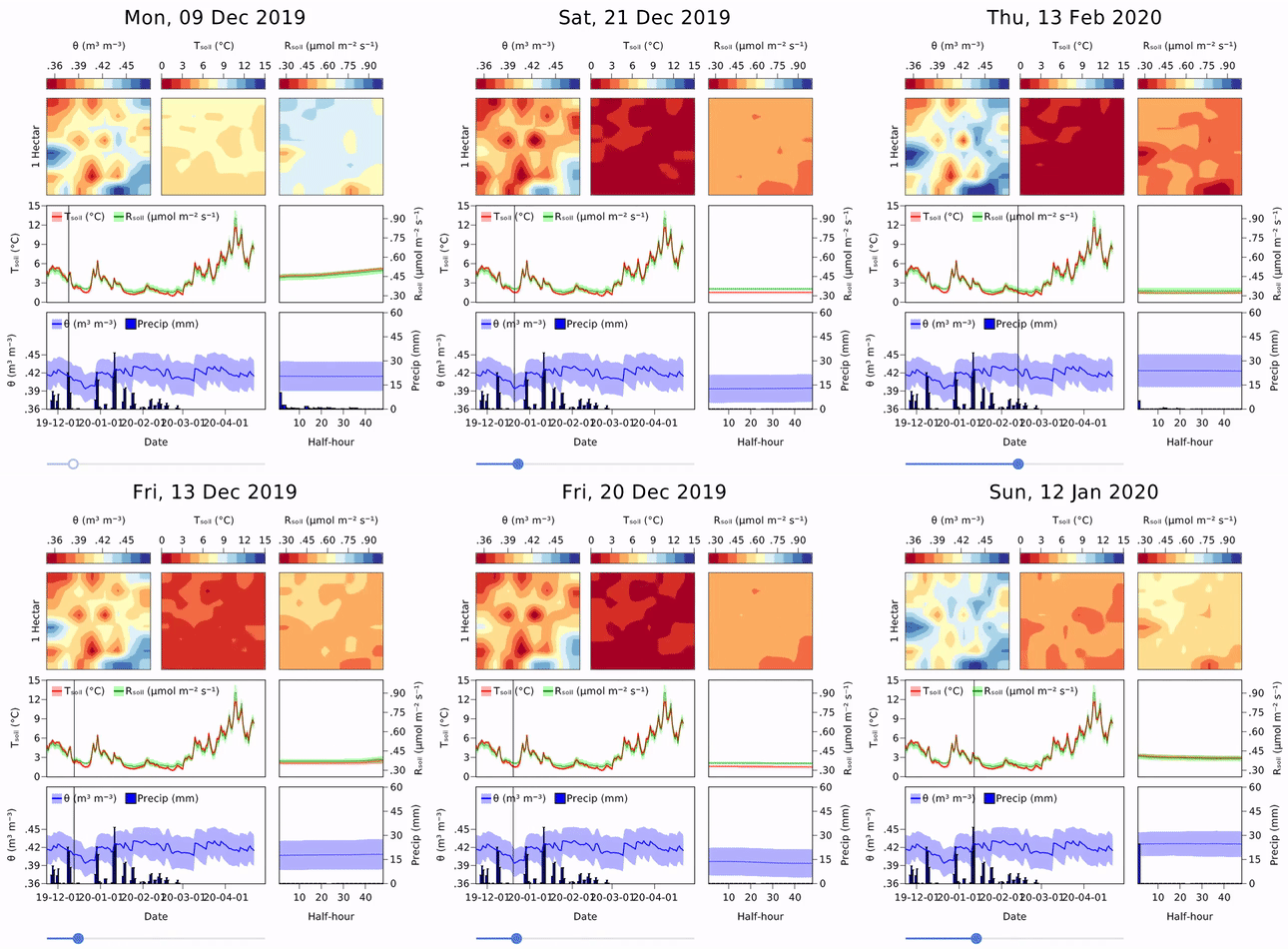
Makie is an interactive data visualization and plotting ecosystem for theJulia programming language,available on Windows, Linux and Mac. The backend packagesGLMakie,WGLMakie,CairoMakieandRPRMakieadd different functionalities: You can use Makie to interactively explore your data and create simple GUIs in native windows or web browsers, export high-quality vector graphics or even raytrace with physically accurate lighting.

The name Makie (we pronounce it Mah-kee) is derived from the japanese wordMaki-e,which is a technique to sprinkle lacquer with gold and silver powder. Data is the gold and silver of our age, so let's spread it out beautifully on the screen!

To learn more, we invite you to visit the documentation atdocs.makie.org.

Citing Makie

If you use Makie for a scientific publication, please acknowledge and support our work by citingour JOSS paperthe following way:

Danisch & Krumbiegel, (2021). Makie.jl: Flexible high-performance data visualization for Julia.
Journal of Open Source Software, 6(65), 3349, https://doi.org/10.21105/joss.03349

BibTeX entry:

@article{DanischKrumbiegel2021,
doi={10.21105/joss.03349},
url={https://doi.org/10.21105/joss.03349},
year={2021},
publisher={The Open Journal},
volume={6},
number={65},
pages={3349},
author={Simon Danisch and Julius Krumbiegel},
title={{Makie.jl}: Flexible high-performance data visualization for {Julia}},
journal={Journal of Open Source Software}
}

orDownload the BibTeX file.

Community Channels

We are onDiscordandDiscourse!Community channels are a great way for you to ask questions and get help. Please join us!

Installation

Choose one or more backend packages:GLMakie(interactive OpenGL in native OS windows),WGLMakie(interactive WebGL in browsers, IDEs, notebooks),CairoMakie(static 2D vector graphics and images) andRPRMakie(raytracing). Each backend re-exports all of Makie.jl so you don't have to install or load it explicitly.

Install:

julia>]
pkg>add GLMakie

Check the installed version:

]st GLMakie

Start using the package:

usingGLMakie

Developing Makie

🔥 Click for more 🔥

Makie and its backends all live in the Makie monorepo. This makes it easier to change code across all packages. Therefore, dev'ing Makie almost works as with other Julia packages, just, that one needs to also dev the sub packages:

]dev--localMakie#local will clone the repository at./dev/Makie
]dev dev/Makie/MakieCore dev/Makie/GLMakie dev/Makie/CairoMakie dev/Makie/WGLMakie dev/Makie/RPRMakie

To run the tests, you also should add:

]dev dev/Makie/ReferenceTests

For more info about ReferenceTests, check out itsREADME

Examples

The following examples are supposed to be self-explanatory. For further informationcheck out the documentation!

A simple parabola

x=1:0.1:10
fig=lines(x, x.^2;label="Parabola",
axis=(; xlabel="x",ylabel="y",title="Title"),
figure=(; size=(800,600), fontsize=22))
axislegend(; position=:lt)
save("./assets/parabola.png",fig)
fig

A more complex plot with unicode characters and LaTeX strings:

Similar to the one on this link

Show Code

x=-2pi:0.1:2pi
approx=fill(0.0,length(x))
cmap=[:gold,:deepskyblue3,:orangered,"#e82051"]
with_theme(palette=(; patchcolor=cgrad(cmap, Alpha=0.45)))do
fig, axis, lineplot=lines(x,sin.(x); label=L"sin(x)",linewidth=3,color=:black,
axis=(; title="Polynomial approximation of sin(x)",
xgridstyle=:dash,ygridstyle=:dash,
xticksize=10,yticksize=10,xtickalign=1,ytickalign=1,
xticks=(-π:π/2:π, ["π","-π/2","0","π/2","π"])
))
translate!(lineplot,0,0,2)#move line to foreground
band!(x,sin.(x), approx.+=x; label=L"n = 0")
band!(x,sin.(x), approx.+=-x.^3/6;label=L"n = 1")
band!(x,sin.(x), approx.+=x.^5/120;label=L"n = 2")
band!(x,sin.(x), approx.+=-x.^7/5040;label=L"n = 3")
limits!(-3.8,3.8,-1.5,1.5)
axislegend(; position=:ct,backgroundcolor=(:white,0.75), framecolor=:orange)
save("./assets/approxsin.png",fig, size=(800,600))
fig
end

Simple layout: Heatmap, contour and 3D surface plot

Show Code

x=y=-5:0.5:5
z=x.^2.+y'.^2
cmap=:plasma
with_theme(colormap=cmap)do
fig=Figure(fontsize=22)
ax3d=Axis3(fig[1,1]; aspect=(1,1,1),
perspectiveness=0.5,azimuth=2.19,elevation=0.57)
ax2d=Axis(fig[1,2]; aspect=1,xlabel="x",ylabel="y")
pltobj=surface!(ax3d, x, y, z; transparency=true)
heatmap!(ax2d, x, y, z; colormap=(cmap,0.65))
contour!(ax2d, x, y, z; linewidth=2,levels=12,color=:black)
contour3d!(ax3d, x, y, z; linewidth=4,levels=12,
transparency=true)
Colorbar(fig[1,3], pltobj; label="z",labelrotation=pi)
colsize!(fig.layout,1,Aspect(1,1.0))
colsize!(fig.layout,2,Aspect(1,1.0))
resize_to_layout!(fig)
save("./assets/simpleLayout.png",fig)
fig
end

Interactive example byAlexisRenchon:

Example fromInteractiveChaos.jl

Sponsors

Förderkennzeichen: 01IS10S27, 2020