Numerical analysis

Numerical analysisstudies differentalgorithmsto getapproximationsfor problems ofmathematical analysis.Approximations are used for the following reasons:
- There are no known ways to solve a problem usingcalculus.Examples for such problems are theNavier–Stokes equations[2][3][4][5]or theThree-body problem
- There is a way to solve a problem using calculus. Getting an exact solution is impractical though, because it requires a long time, or many resources. An example for this is calculatingpower series.
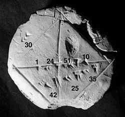
One of the earliest known uses of numerical analysis is aBabylonianclaytablet,which approximates thesquarerootof2.In a unit square, the diagonal has this length. Being able to compute the sides of a triangle is extremely important, for instance, incarpentryandconstruction.[6]
Numerical analysis continues this long tradition of practical mathematical calculations. Much like the Babylonian approximation of,modern numerical analysis does not seek exact answers, because exact answers are often impossible to obtain in practice. Instead, much of numerical analysis is concerned with obtaining approximate solutions while maintaining reasonable bounds on errors.
Numerical analysis naturally finds applications in all fields ofengineeringand the physical sciences,[7]but in the 21st century, the life sciences and even the arts have adopted elements of scientific computations. Ordinarydifferential equationsappear instar movement;optimizationoccurs in portfolio management;numerical linear algebrais important for data analysis;[8][9][10]stochasticdifferential equations[11][12][13][14][15]andMarkov chains[16]are essential in simulating living cells formedicineandbiology.[17]
Computersgreatly helped this task. Before there were computers, numerical methods often depended on handinterpolationin large printed tables. Since the mid 20th century, computers calculate the required functions instead.[18]These same interpolation formulas nevertheless continue to be used as part of the softwarealgorithmsfor solvingdifferential equations.[19][20][21]
Famous numerical software
[change|change source]In order to support numerical analysts, many kinds of numericalsoftwarehas been created:
- MatLab[22][23][24]- made byMathWorks
- GNU Octave,Scilab-open sourceversions of MATLAB
- SageMath[25]
- SciPy[26][27][28]
- Wolfram Mathematica[29][30][31][32]- made byWolfram Research
References
[change|change source]- ↑"Photograph, illustration, and description of theroot(2)tablet from the Yale Babylonian Collection ".Archived fromthe originalon 2012-08-13.Retrieved2012-03-25.
- ↑Constantin, P., & Foias, C. (1988). Navier-stokes equations. University of Chicago Press.
- ↑Temam, R. (2001). Navier-Stokes equations: theory and numerical analysis (Vol. 343).American Mathematical Society.
- ↑Foias, C., Manley, O., Rosa, R., & Temam, R. (2001). Navier-Stokes equations and turbulence (Vol. 83).Cambridge University Press.
- ↑Girault, V., & Raviart, P. A. (2012). Finite element methods for Navier-Stokes equations: theory and algorithms (Vol. 5). Springer Science & Business Media.
- ↑The New Zealand Qualification authority specifically mentions this skill in document 13004 version 2, dated 17 October 2003 titledCARPENTRY THEORY: Demonstrate knowledge of setting out a building
- ↑Garcia, A. L. (2000). Numerical methods for physics. Englewood Cliffs, NJ: Prentice Hall.
- ↑Demmel, J. W. (1997). Applied numerical linear algebra.SIAM.
- ↑Ciarlet, P. G., Miara, B., & Thomas, J. M. (1989). Introduction to numerical linear algebra and optimization. Cambridge University Press.
- ↑Trefethen, Lloyd; Bau III, David (1997). Numerical Linear Algebra (1st ed.). Philadelphia:SIAM.
- ↑Kloeden, P. E., & Platen, E. (2013). Numerical solution of stochastic differential equations (Vol. 23). Springer Science & Business Media.
- ↑Oksendal, B. (2013). Stochastic differential equations: an introduction with applications. Springer Science & Business Media.
- ↑Mao, X., & Yuan, C. (2006). Stochastic differential equations with Markovian switching. Imperial College Press.
- ↑Mao, X. (2007). Stochastic differential equations and applications.Elsevier.
- ↑Platen, E. (1999). An introduction to numerical methods for stochastic differential equations. Acta Numerica, 8, 197-246.
- ↑Behrends, E. (2000). Introduction to Markov chains (Vol. 228). Braunschweig/Wiesbaden: Vieweg.
- ↑Tass, P. A. (2007). Phase resetting in medicine and biology: stochastic modelling and data analysis. Springer Science & Business Media.
- ↑Brezinski, C., & Wuytack, L. (2012). Numerical analysis: Historical developments in the 20th century. Elsevier.
- ↑Iserles, A. (2009). A first course in the numerical analysis of differential equations. Cambridge University Press.
- ↑Ames, W. F. (2014). Numerical methods for partial differential equations. Academic Press.
- ↑M. Nakao, M. Plum, Y. Watanabe (2019) Numerical Verification Methods and Computer-Assisted Proofs for Partial Differential Equations (Springer Series in Computational Mathematics).
- ↑Quarteroni, A., Saleri, F., & Gervasio, P. (2006). Scientific computing with MATLAB and Octave. Berlin: Springer.
- ↑Gander, W., & Hrebicek, J. (Eds.). (2011). Solving problems in scientific computing using Maple and Matlab®. Springer Science & Business Media.
- ↑Barnes, B., & Fulford, G. R. (2011). Mathematical modelling with case studies: a differential equations approach using Maple and MATLAB. Chapman and Hall/CRC.
- ↑Zimmermann, P., Casamayou, A., Cohen, N., Connan, G., Dumont, T., Fousse, L.,... & Thiéry, N. M. (2018). Computational mathematics with SageMath. Society for Industrial and Applied Mathematics.
- ↑Jones, E., Oliphant, T., & Peterson, P. (2001). SciPy: Open source scientific tools for Python.
- ↑Bressert, E. (2012). SciPy and NumPy: an overview for developers. "O'Reilly Media, Inc.".
- ↑Blanco-Silva, F. J. (2013). Learning SciPy for numerical and scientific computing. Packt Publishing Ltd.
- ↑Maeder, R. E. (1991). Programming in mathematica. Addison-Wesley Longman Publishing Co., Inc..
- ↑Stephen Wolfram. (1999). The MATHEMATICA® book, version 4. Cambridge University Press.
- ↑Shaw, W. T., & Tigg, J. (1993). Applied Mathematica: getting started, getting it done. Addison-Wesley Longman Publishing Co., Inc..
- ↑Marasco, A., & Romano, A. (2001). Scientific Computing with Mathematica: Mathematical Problems for Ordinary Differential Equations; with a CD-ROM. Springer Science & Business Media.
Researchers
[change|change source]Related pages
[change|change source]| Mediafrom Commons | |
| Quotationsfrom Wikiquote | |
| Textbooksfrom Wikibooks | |
Further reading
[change|change source]- Higham, Nicholas J. (1996). Accuracy and Stability of Numerical Algorithms.Society for Industrial and Applied Mathematics.
- Gautschi, W. (1997). Numerical analysis. Springer Science & Business Media.
- Leader, Jeffery J. (2004). Numerical Analysis and Scientific Computation. Addison Wesley.
- Quarteroni, A., Sacco, R., & Saleri, F. (2010). Numerical mathematics. Springer Science & Business Media.
- Stoer, J., & Bulirsch, R. (2013). Introduction to numerical analysis. Springer Science & Business Media.
- Conte, S. D., & De Boor, C. (2017). Elementary numerical analysis: an algorithmic approach.Society for Industrial and Applied Mathematics.
- Greenspan, D. (2018). Numerical Analysis. CRC Press.
- Linz, P. (2019). Theoretical numerical analysis. Courier Dover Publications.


